Phylogenetics

The study of evolutionary relationships among biological entities

Warning

Be sure to use the phylo Codespace when initiating VM for this practical.

Objectives

By the end of this practical you should:

• Understand the relationship between genetic relatedness and transmission events.
• Know how to reconstruct and interpret a phylogenetic tree
• Understand how time and spatial diffusion of an epidemic is inferred from a phylogeny

Introduction

In the lecture, we saw how epidemiological processes leave a measurable imprint on pathogen genomes sampled from infected individuals. These processes can be recovered from genetic data sampled at different times and places, using statistical inference methods that take into account the sequences’ shared ancestry.

In this practical session, we will reconstruct and interpret the Influenza A H1N1 2009 (H1N1/09) epidemic in England, based on a set of viral sequences isolated during the outbreak.

We will identify transmission chains of H1N1/09, reconstruct their migration patterns, estimate the number of independent introductions in England, and infer the time and geographical location of these introduction events. In order to do so, we will apply the following procedure:

1. We will reconstruct the phylogeny of influenza genomes sampled in England and other countries where H1N1 infections were diagnosed.
2. We will apply a molecular clock model to the data in order to fit the phylogeny to real time scales.
3. We will infer the migration patterns of H1N1 into and within England using Bayesian Markov chain Monte Carlo (MCMC) phylogeographic inference.

---

Section 1 - Phylogenetic reconstruction

We will use the tool Alv to view genetic sequence files and build a maximum-likelihood (ML) phylogenetic tree.

Optional: view the alignment in a GUI instead

If you'd rather inspect the alignment visually, you can use **aliview** ([download](https://ormbunkar.se/aliview/downloads/)). Download **H1N1.flu.2009.fas** from vscode, then **File > Open File** and select it.

The file ‘H1N1.flu.2009.fas’ is a multi-FASTA file containing 50 full-length influenza A H1N1/09 genomes. These nucleotide sequences correspond to influenza viruses sampled in Canada (n = 5), China (n = 3), England (n = 23), Mexico (n = 4), Peru (n = 1), and the United States of America (USA; n = 14) between April and June 2009. The sequences are 12,735 nucleotides long.

We will use Alv to manually inspect the FASTA file:

Activate the correct environment with conda activate phylo.

cd ~/data/phylogenetics/
alv -t dna -k --color-scheme terminal H1N1.flu.2009.fas | less -R

Important

To infer the phylogenetic relationship of a set of sequences, these need to be ‘aligned’. That is, nucleotide positions need to be arranged in columns to ensure that we compare homologous positions to one another. In evolutionary biology, homology means similarity due to descent from a common ancestor. Two genes are homologous if they descend from an ancestral gene. Likewise, two nucleotides in different sequences are homologous if they correspond to the same nucleotide position in the ancestral gene. Note that two objects can be ‘similar’ without being ‘identical’. The sequences shown here have been aligned but if your data is not, it will need to be aligned. This can be done in AliView, as well as in other programs including MUSCLE, ClustalW and our recommendation MAFFT. This has been done before because these steps can take a while to run.

The sequence alignment is displayed as a matrix, where rows correspond to viral samples and columns to nucleotide positions (see Figure 1). Cells are coloured by type of nucleotides (A, C, G or T) and missing information, or gaps, are indicated by a dash (“-“).

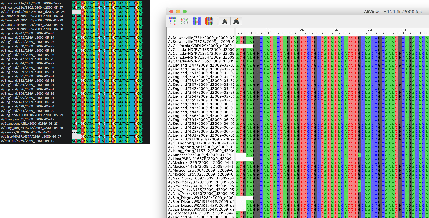
The unique identifier of the sequences is shown at the left hand side of the nucleotide matrix and contains the strain name (e.g. A/England/247/2009) followed by the date of sampling (e.g. d2009-05-31) in the format dYYYY-MM-DD.

In the matrix, we can spot ‘rare’ nucleotide substitutions present in one or more sequences (scroll along the sequence alignment to spot some). These single nucleotide polymorphisms (SNPs) allow us to identify viruses that are genetically related (they share a common SNP) and infer epidemiological linkage between them. If viruses sampled from different individuals have the same SNPs, we can assume that they form a specific strain infecting these individuals. This is the property we use to reconstruct transmission chains from a phylogenetic tree.

Tree reconstruction

IQ-Tree [1] is a freely available software used to reconstruct phylogenetic relationships between individuals using a maximum-likelihood (ML) approach. This approach takes into account a substitution model to assess the probability of particular mutations. You can also perform bootstrapping, a method for validating the tree by repeating the analysis a specified number of times to produce pseudoreplicates. This acts as a support for the tree topology of the final tree that is produced by calculating the number of pseudoreplicates in which a given node of a tree is found.

Open your command-line terminal and navigate to the folder containing the H1N1.flu.2009.fas sequence file.

Run the following command (This may take a few minutes to complete):

iqtree -m GTR+G -s H1N1.flu.2009.fas -bb 1000 

• iqtree: This will run iqtree on the command-line and uses the following parameters:
• m GTR+G: This sets the substitution model to be used. We are using GTR (generalised time reversible) with a gamma distribution.
• s H1N1.flu.2009.fas: This is your input file. --bb 1000: This specifies the number of bootstrap runs.

Once the software has finished running, the file H1N1.flu.2009.fas.treefile will contain the ML tree with bootstrap supports.

Download this file from the codespace, then upload it to iTOL to view the phylogeny.

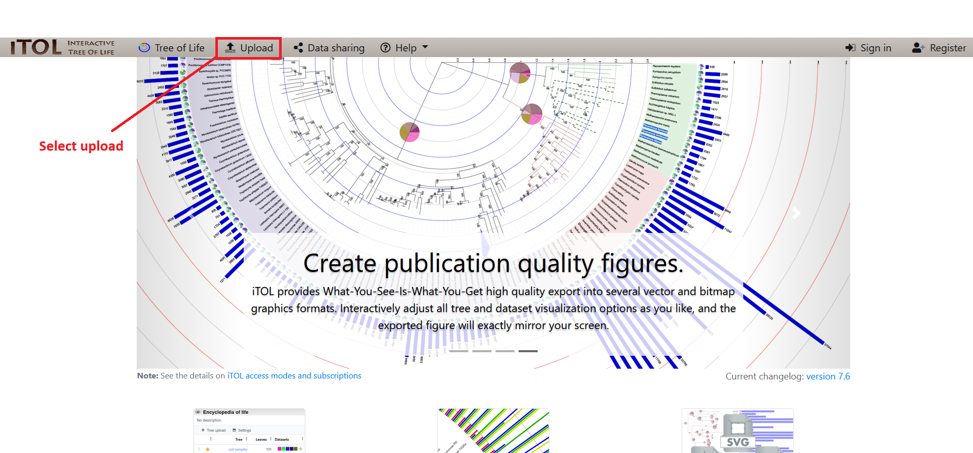
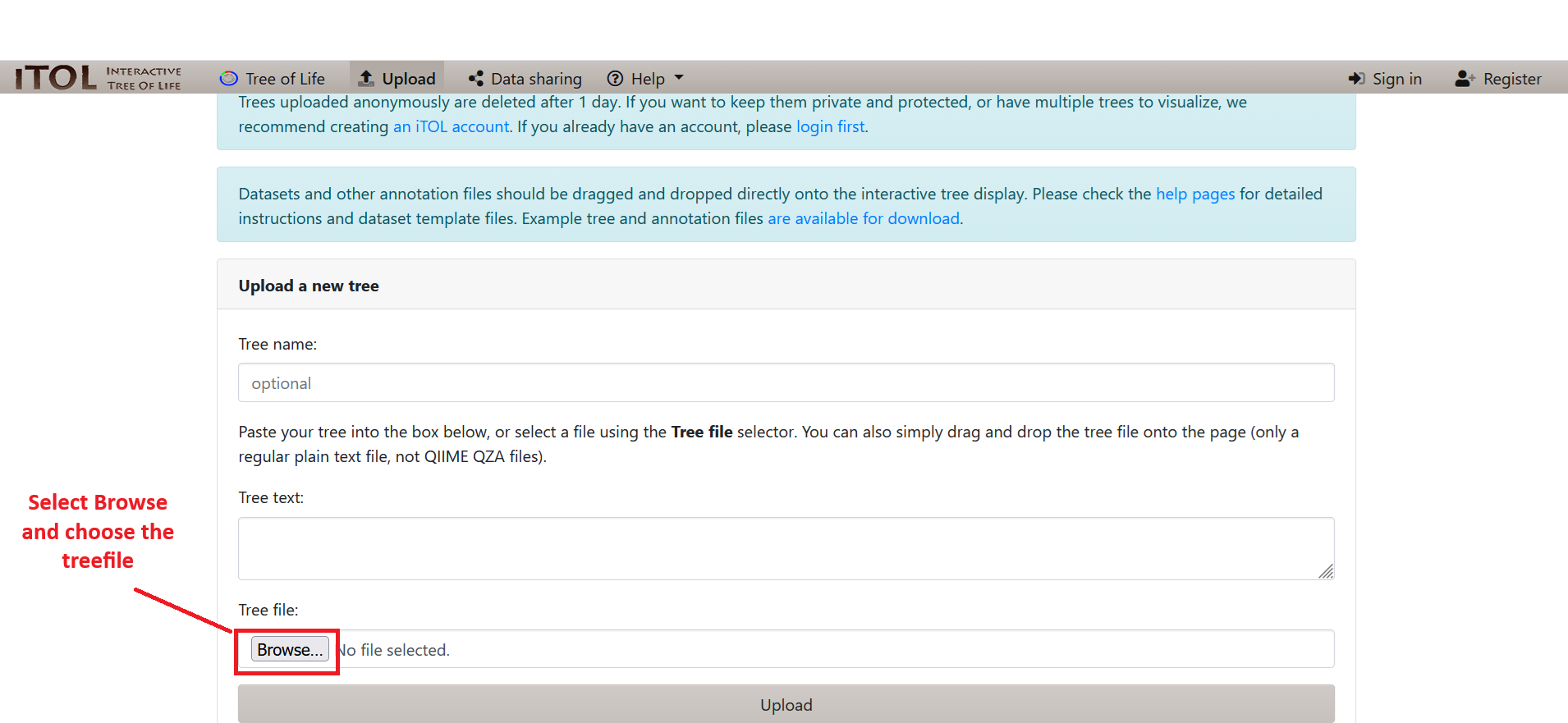
In iTOL, open the Advanced tab in the control panel, and find the Bootstraps / metadata option in the Branch metadata display section. Set it to Display, then choose the bootstrap values as the data source. The support value for each node will now appear on the branches. You can also increase the font size to make it clearer and addign a Label background to make it even more clearer. iTOL sorts clades by size automatically, giving laddered, top-to-bottom order. If the tree doesn't look sorted, check that Leaf sorting is enabled in the display options.

Note

Note. Many of the values shown are low (the scale is 0 [no support] to 100 [full support]). Typically values over 70% (in this case a bootstrap value of 70) are taken as showing strong support. Low values here may suggest that you need to change the substitution model or run the analysis with more bootstrap runs. For the purposes of time for this exercise, we will continue with the trees produced here.

Tree Interpretation

Take a few minutes to familiarize yourself with the tree.

Reminder

The components of a phylogenetic tree are shown in Figure 3. The sequences, or taxa (plural for taxon), are positioned at the end of the external branches. Related sequences are linked by a node (their most recent common ancestor). Two or more sequences descending from a node form a ‘clade’ (or cluster). The length of a branch represents the genetic distance between two nodes or between a node and a taxon, i.e., the number of mutations accumulated since divergence. The root corresponds to the common ancestor of all the taxa.

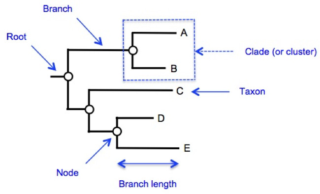
Since the sequences represent viruses sampled from different individuals, a clade in the tree corresponds to a transmission chain. The number of sequences in a clade reflects the number of infections sampled from that transmission chain. The root of the tree corresponds to the origin of the epidemic.

Now we can upload an annotation file to view the england strains highlighted as red, which has been provided for you. This file is called first_tree_anno.txt, and to upload it we select Datasets in the iTOL control panel, and choose Upload annotation files.

After looking at your tree with iTOL, can you answer these questions:

Question

Q1Answer

How many times was H1N1/2009 introduced in England during the outbreak?

Q1. The viruses sampled in England form 3 distinct clades, suggesting 3 introduction events (colored in red in the figure below). The first one involves 18 cases (top of the tree), the second 2 cases (A/England/247/2009 and A/England/251/2009), and the third one 3 cases (A/England/247/2009, A/England/312/2009, and A/England/415/2009).

Question

Q2Answer

What is/are the most likely geographical origins of the English strain(s)? (Take the sampling dates into account in your reasoning)

Q2. Cluster 1 is closest to a Canadian clade made of 4 cases. The two clades share a recent common ancestor located at node 1. All Canadian isolates were sampled in April 2009, while the viruses in the English Cluster 1 were sampled in May or June the same year. We can, therefore, assume that the strain migrated from the Americas to Europe (as we know it did…). We can also infer precedence of the Canadian outbreak by the fact that the Canadian sequences are genetically more similar to the common ancestor (node 1) than the English ones, as indicated by shorter branch lengths.

Cluster 2 is closest to a Canadian isolate (A/Toronto/3141/2009). Their common ancestor is located at node 2. The Toronto isolate predates the English ones, suggesting an introduction from Canada.

Cluster 3 is closest to a US isolate (A/New York/3532/2009). Their common ancestor is located at node 3. Again, we can conclude from the time of sampling and branch lengths that Clade 3 was imported from the US.

Dating the Introduction(s) of H1N1/09 in England

We will now estimate the time frame of these migration events. This time frame can be inferred from the rate at which mutations are accumulated in gene sequences. If, for instance, two sequences differ by 4 mutations and their rate of evolution is known to be around one substitution per nucleotide position per year, then 2 years have elapsed since they diverged from their common ancestor (i.e., 1 substitution x 2 years x 2 sequences = 4 mutations).

The first step of this procedure involves testing whether the genomes in the tree have evolved at a constant rate over time or not. This is called testing the molecular clock hypothesis.

If the molecular clock is constant or strict, the genetic distance between two sequences will be proportional to the time since these sequences last shared a common ancestor (as in the example given above). If the molecular clock is not constant, the correlation between genetic distance and time since divergence is weaker. The molecular clock is then said to be relaxed. Assuming a strict or relaxed molecular clock will have an impact on the dating of phylogenetic nodes. We will, therefore, test the molecular clock hypothesis before dating the tree.

Molecular Clock Testing

Molecular clock testing is normally done with a GUI tool called TempEst, but to keep everything on the command line we'll reproduce its core function which is root-to-tip regression, with a custom Python script, roottotip.py.

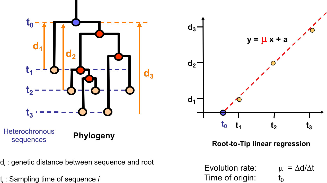
What is it doing? The script tests the ‘temporal signal’ of the phylogeny: whether there is enough genetic change between sampling times to reconstruct a statistical relationship between genetic divergence and time, which is the essence of a molecular clock in your data.

How does it work? It performs a ‘root-to-tip’ linear regression, a simple diagnostic for molecular clock models. It plots the genetic divergence of each sequence (the sum of branch lengths from that tip back to the root) against its sampling time (Figure 3). A linear trend with few residuals indicates evolution follows a strict molecular clock. The same trend with greater scatter suggests a relaxed molecular clock model is more appropriate. No trend at all means the data contains little temporal signal and is unsuitable for molecular-clock inference.

The sampling date of each sequence is encoded at the end of its name, preceded by the suffix _d, in the format YYYY-MM-DD. For instance, A/Lima/WRAIR1687P/2009_d2009-06-27 was sampled on the 27th of June 2009. The script reads these dates automatically.

Before running the regression on the ML tree, we first need to install two dependencies required by the analysis. This is a common situation you may encounter in your own work, where additional software packages are needed to run a tool.

Install the required dependencies with:

pip install dendropy
pip install matplotlib

Once both dependencies have been installed, we can run the root-to-tip regression on the ML tree generated earlier:

python3 roottotip.py H1N1.flu.2009.fas.treefile --prefix _d --seqlen 12735 --out roottotip.png

This will perform the regression analysis and save the resulting plot as roottotip.png.

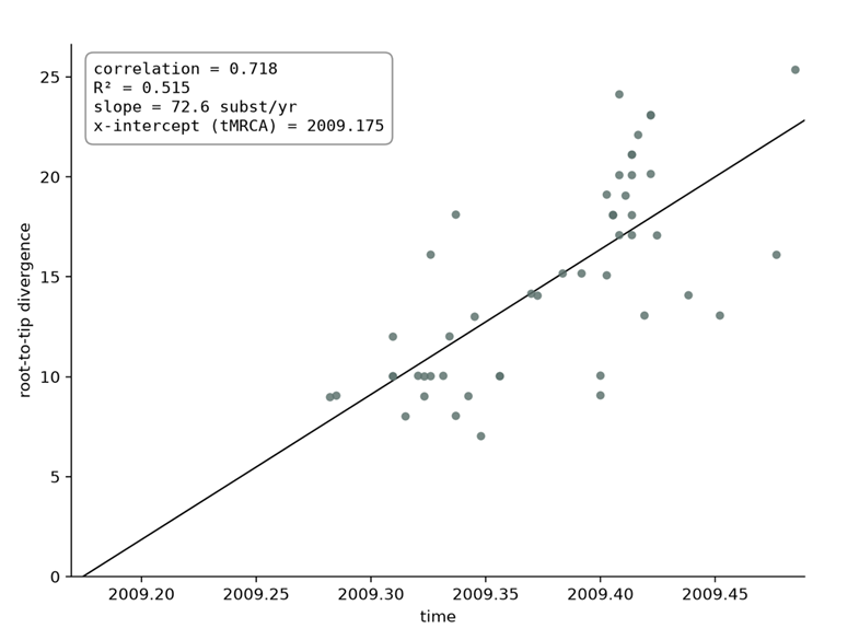
This does the equivalent of Tempest’s Parse Dates (prefix _d, format yyyy-MM-dd) and Best-fitting root steps automatically: it parses each tip’s date, finds the root position that maximises the fit, runs the regression, and writes the plot to roottotip.png (open it from the file browser). It also prints the summary statistics to the terminal, for both the as-is root and the best-fitting root — read the best-fitting root values:

• Date range: the maximum time interval between two sampled sequences.
• Slope: the slope of the regression line; the rate of evolution, average number of nucleotide substitutions per site per year.
• X-intercept (tMRCA): the time at which the population had no genetic diversity, i.e. the time of the most recent common ancestor of the sampled population.
• Correlation coefficient: the strength of the relationship between time and accumulated mutations (range -1 to 1). A positive value means genetic divergence increases with time; a value near 0 means no relationship.
• R²: how close the data sit to the regression line, the proportion of variation in genetic divergence explained by a strict molecular clock.

Question

Q3Answer

Can we assume that the rate of evolution of the viruses in the phylogeny is constant over time (i.e., that the molecular clock is strict)?

The root-to-tip linear regression plot shows a positive correlation between time and divergence (correlation coefficient = 0.71; see the figure and statistics in the terminal). This suggests that the phylogeny has sufficient temporal signal to conduct a molecular clock analysis on this dataset.

However, there is a certain degree of scatter from the regression line, and only 51% of the variation in genetic divergence is explained by a strict molecular clock hypothesis (R squared = 0.51). We will, therefore, assume significant variation from a strict molecular clock in this dataset and opt for a relaxed molecular clock (i.e., the rate of evolution varies over time and across lineages). This is despite a relatively short sampling interval (about 3 months) and moderate genetic diversity in the sampled population.

Dating Migration Events

Now that the properties of the molecular clock in our dataset have been established, we will estimate the time(s) at which H1N1/09 was introduced in England.

Reminder

In a ‘classic’ phylogenetic tree, branch lengths reflect as the number of nucleotide substitutions per site. Rates of evolution are expressed as the number of substitutions per site per unit of time. By dividing the length of a branch by the rate of evolution, we end up with a tree where branch lengths represent time units. A branch therefore represents the time elapsed between two nodes. Or, in our case, the time elapsed between two transmission events.

The reconstruction of dated phylogenetic trees is computationally intense and could not be achieved within the time imparted for this practical. A dated H1N1/09 phylogeny was therefore built prior to the session, under the appropriate molecular clock model, using the Bayesian MCMC approach implemented in the software BEAST v.1.8 [3]. The resulting dated tree is in your folder under the name H1N1.flu.2009.mol_clock.tre. A more detailed example of how to set up a BEAST v1.8. analysis, including producing the input files and analysing the output is shown in the Appendix.

How does it work? Each tip of the tree has a known time, given by the sampling date of the sequence. Internal nodes are given arbitrary starting times consistent with their order in the tree (from the tips to the root). An additional parameter, the evolution rate, is used to scale these times into expected number of nucleotide substitutions per site. Markov chain Monte Carlo integration is then used to summarise the probability density function of a model tested against the data, providing a representative sample of parameter values of the chosen model. The model includes the tree topology, the times of internal nodes and the evolution rate.

We will use the iTOL again to display the dated tree and its annotations.

Open iTOL from the url again.

Upload the file H1N1.flu.2009.mol_clock.2.tre in the same way as before.

You can also upload the file second_tree_anno.txt in the Datasets section to highlight the England strains, this will ease comparison. The dated tree should be very similar to the ML tree you reconstructed in Session 1. However, in this tree, the branch lengths represent days rather than genetic distances.

Once again we can select Advanced and choose Bootstraps / metadata inside the control panel, but this time there is a lot more options to choose from, such as height which is the estimated age or location.prob which is the probability of the location given. Lets have a look at height and make sure to select Text instead of Symbol to view the actual numbers. You can increase the font size to make it clearer and add a label background. You can now answer the following question. Here, Cluster 1 is located towards the bottom of the tree, Cluster 2 is in the middle and Cluster 3 is at the top, all shown in red!

Question

Q4Answer

According to the molecular clock dating, what are the date(s) of introduction of H1N1/09 in England ? Tip: If mental arithmetic is not your thing, you can use the 2009 calendar provided as Appendix to back-calculate the date of the nodes.

Note dates may vary due to rounding! The most recent viral sequence (A/Lima/WRAIR1687P/2009) was sampled on 27/06/2009. The ancestral node of Cluster 1 has an age of ~63 days prior to the most recent sample. The estimated date of the first introduction of H1N1/09 in England is thus 25/04/2009.

The ancestral node of Cluster 2 has an age of ~58 days prior to the most recent sample. The estimated date of the second introduction of H1N1/09 in England is thus 01/05/2009.

The ancestral node of Cluster 3 has an age of ~41 days prior to the most recent sample. The estimated date of the third introduction of H1N1/09 in England is thus 18/05/2009.

Identifying the geographical origin(s) of the H1N1/09 strains imported in England

We will finally reconstruct the migration pathways of these H1N1/09 strains.

Reminder

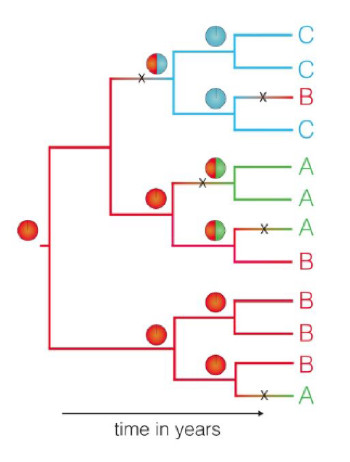
When individuals are infected in one location and then move to another, or infect someone whilst travelling, this is apparent as a “change” in the location ascribed to one branch of the tree. These changes in location along a phylogenetic tree can be inferred from the location values at the tips and the shape of the tree (see Figure 4). To do so, a model of location exchange process is fitted to the data and the most likely location of the viral strain positioned at the nodes of the tree, together with its probability, can be estimated using a MCMC sampling procedure similar to the one used in Section 2.

This approach was applied to the H1N1/09 phylogeny, using an asymmetric continuous-time Markov chain [5], as implemented in the program BEAST. The asymmetric model uses separate parameters for forward and reverse rates of movement between each pair of locations. The tree file we used for the molecular clock analysis (H1N1.flu.2009.mol_clock.2.tre) also contains the result of the inferred migration patterns.

On the control panel we will now selection location in the control panel under Bootstraps / metadata to see the most likely location of the ancestral virus.

To display the posterior probability of the most likely node location, select Location.prob once again selecting Text and changing the font-size in the control panel.

Question

Q5Answer

Which country is the most likely source of the H1N1/09 epidemic? What is the probability of that location?

The most likely location state at the root of the tree is the US (posterior probability: 0.84).

Question

Q6Answer

Where were the English strains of H1N1/09 imported from? How confident are we? How does your answer compare to that of Q4?**

• The location at the node from which Cluster 1 is branching off (node 1 in the figure shown with the answer to Q1) is the US (posterior probability: 0.55).
• The location at the node from which Cluster 2 is branching off (node 2 in the figure shown with the answer to Q1) is Canada (posterior probability: 0.48).
• The location state at the node from which Cluster 3 is branching off (node 3 in the figure shown with the answer to Q1) is the US (posterior probability: 0.87).

The geographical origin of the founder viruses is consistent for Cluster 2 and 3. However, for Cluster 1, the tree topology suggests relatedness with a Canadian cluster while the phylogeographic reconstruction places the founder virus of that cluster in the US. The most likely explanation is that the English and Canadian viruses were both imported from the US.

References

1. A. Stamatakis: 'RAxML Version 8: A tool for Phylogenetic Analysis and Post-Analysis of Large Phylogenies'. Bioinformatics, 2014
2. A. Rambaut, T. T. Lam, L. Max Carvalho, and O. G. Pybus, ‘Exploring the temporal structure of heterochronous sequences using TempEst (formerly Path-O-Gen)’, Virus Evol., vol. 2, no. 1, p. vew007, Jan. 2016.
3. A. J. Drummond, M. A. Suchard, D. Xie, and A. Rambaut, ‘Bayesian Phylogenetics with BEAUti and the BEAST 1.7’, Mol. Biol. Evol., vol. 29, no. 8, pp. 1969–1973, Jan. 2012.
4. N. R. Faria et al., ‘The early spread and epidemic ignition of HIV-1 in human populations’, Science, vol. 346, no. 6205, pp. 56–61, Mar. 2014.
5. P. Lemey, A. Rambaut, A. J. Drummond, and M. A. Suchard, ‘Bayesian phylogeography finds its roots’, PLoS Comput. Biol., vol. 5, no. 9, p. e1000520, Sep. 2009.

Extra

Like other practicals we also have a task set out for this practical, once again the Tasks tab at the top and the Phylo task is the one related to this practical. If you feel confident you can give it a go.

Appendix

Phylogenetic Tree Building with BEAST

Important

You dont need to run this step as it takes a while, this is just incase you wish to attempt it yourself.

(Note: This example is for initializing a BEAST v.1.8 analysis; BEAST2 has a different interface.)

1. Creating a BEAST Input File Using BEAUti

You can download BEAST and Beauti here. Once downloaded you first open Beauti

1.1. Load the FASTA sequence file H1N1.flu.2009.fas by clicking the + button or going to File > Open….

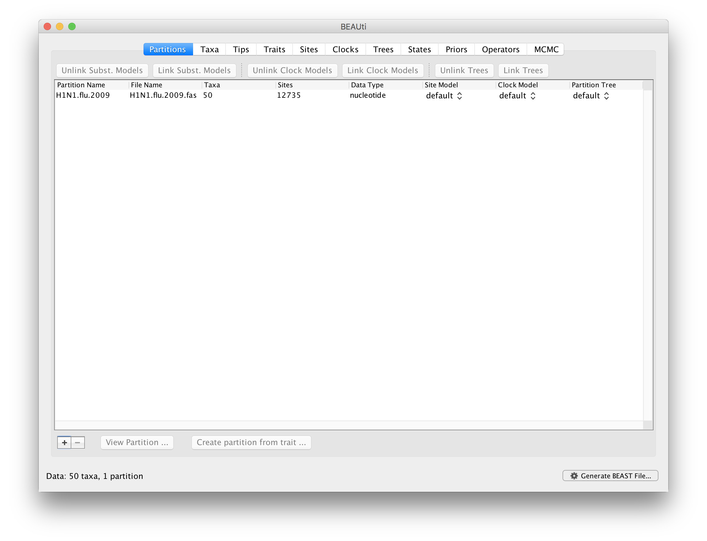
This first will give you information on the number of taxa (50), the number of sites (12735), and the data type (nucleotide).

If you want to partition the data, i.e. if you have samples that you know are from different populations or lineages, you can go onto the ‘Taxa’ tab and set these partitions. This will allow you to specify whether these groups are monophyletic as well as divergence dates between groups. For this exercise, we will not assume any partitioning of samples.

1.2. Attach a date to each sample.

This can be done in the same way as was shown in TempEst: In the Tips tab, tick the box for Use tip dates, and then click on Parse Dates. In the Parse Dates for Taxa window, select the following options:

• The date is given by a numerical field in the taxon label that is defined by a prefix and its order (Order: Last; Prefix: _d)
• Parse as a calendar date (Date format: yyyy-MM-dd)

Alternatively, you can create a tab-delimited file (.txt) with two columns corresponding to the taxa names and sample dates, and use Import Dates.

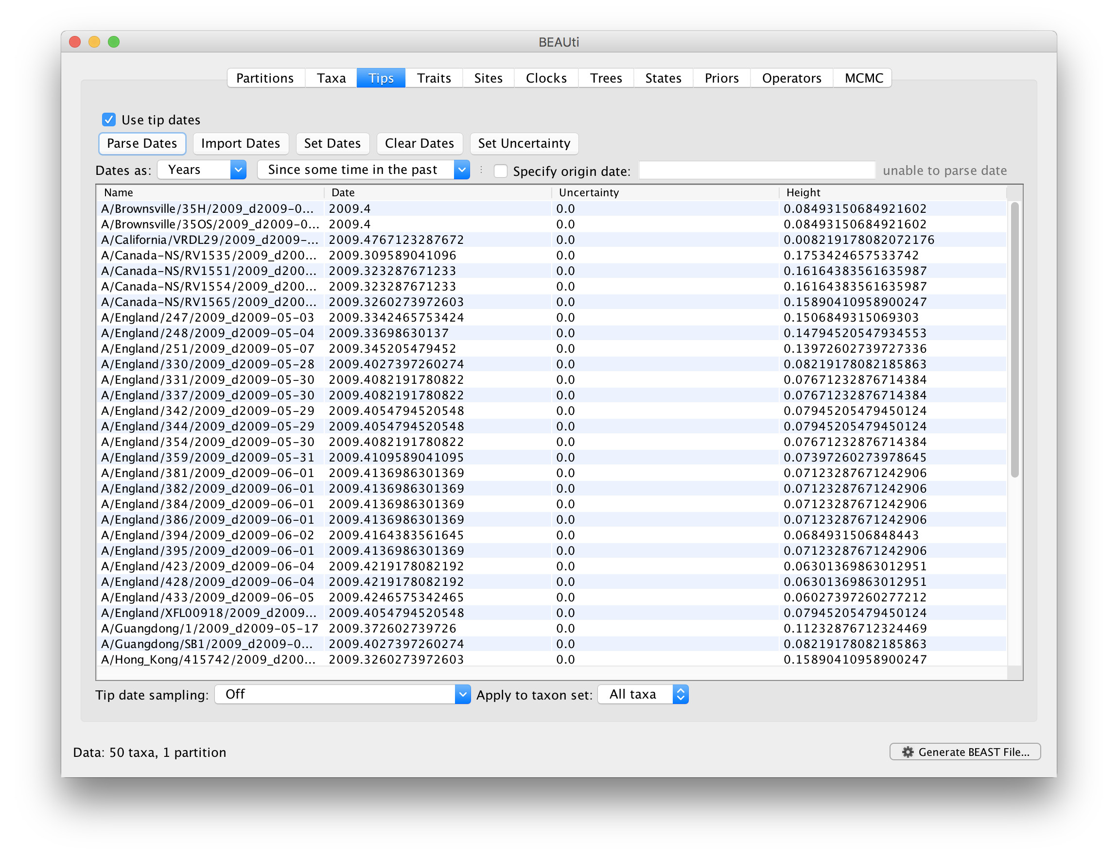
1.3. Set the location for each sample

To attach further traits to each sample, such as location, in the Traits tab, click on Import Traits and open a tab-delimited file (.txt) with two columns corresponding to the taxa names and location (or characteristic of choice).

1.4. Set a site (substitution) model.

This allows us to substitution and site heterogeneity models. The rate and likelihood of base substitution over the genome will be variable so we will set some parameters to describe the model of substitution. We will set the substitution model to GTR – Generalized Time Reversible model – as this is the most frequently used model and allows for variable base frequencies. It is also reversible (i.e. T->A same rate as A->T). We can also set the site heterogeneity model, i.e. the frequency of each site to a Gamma distribution with 4 categories.

In the Sites tab, select GTR from the ‘Substitution model’ dropdown box. We will set the ‘Site Heterogeneity model’ as ‘Gamma’ with 4 categories.

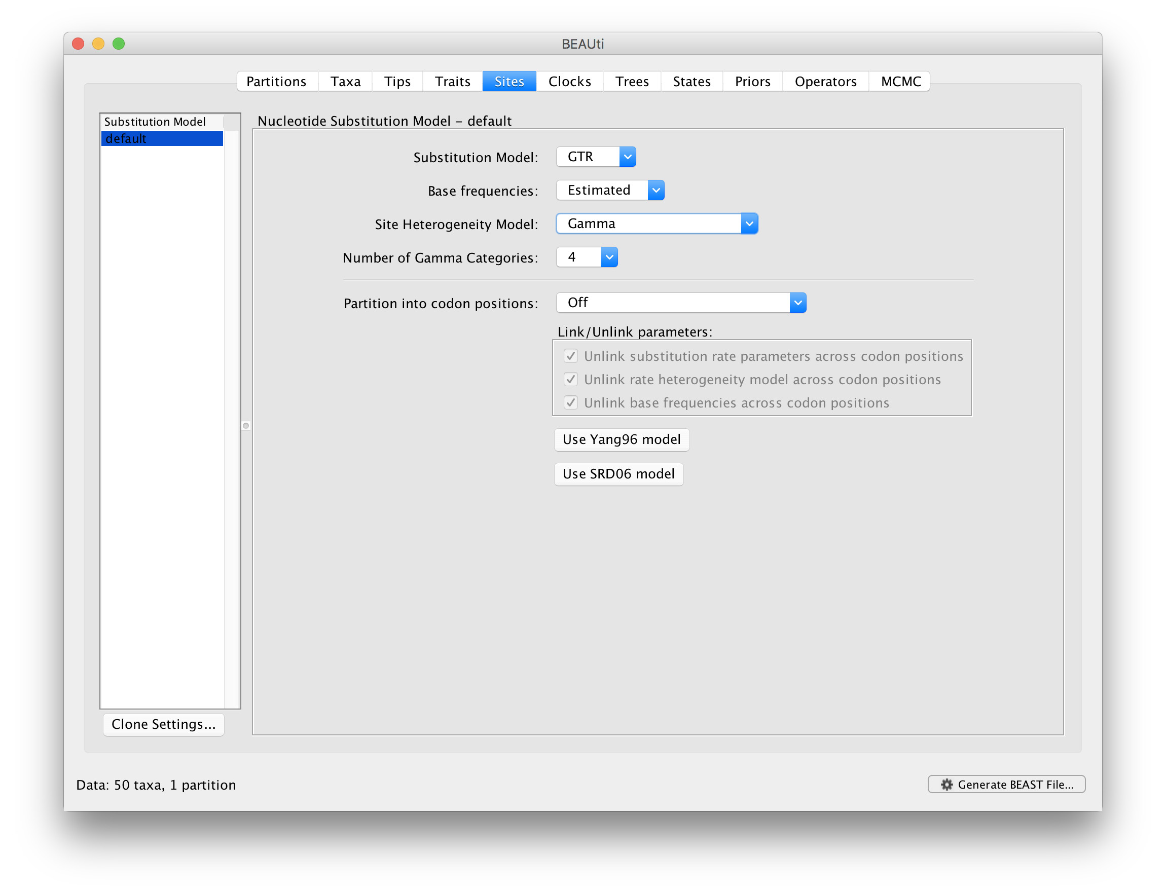
1.5 Set a clock model. The ‘Clocks’ tab will allow us to set the molecular clock for mutations along each branch of the tree. If we set this to ‘Strick Clock’ this specifies that the mutation rate along each branch will be invariable. As we have shown in the TempEst analysis that our data varies significantly from a strict molecular clock, we will select a relaxed clock to allow for rate variation across branches in our tree.

In the Clocks tab, select ‘Uncorrelated relaxed clock’ from the ‘Clock Type’ dropdown box and keep the ‘Relaxed Distribution’ option as ‘Lognormal'.

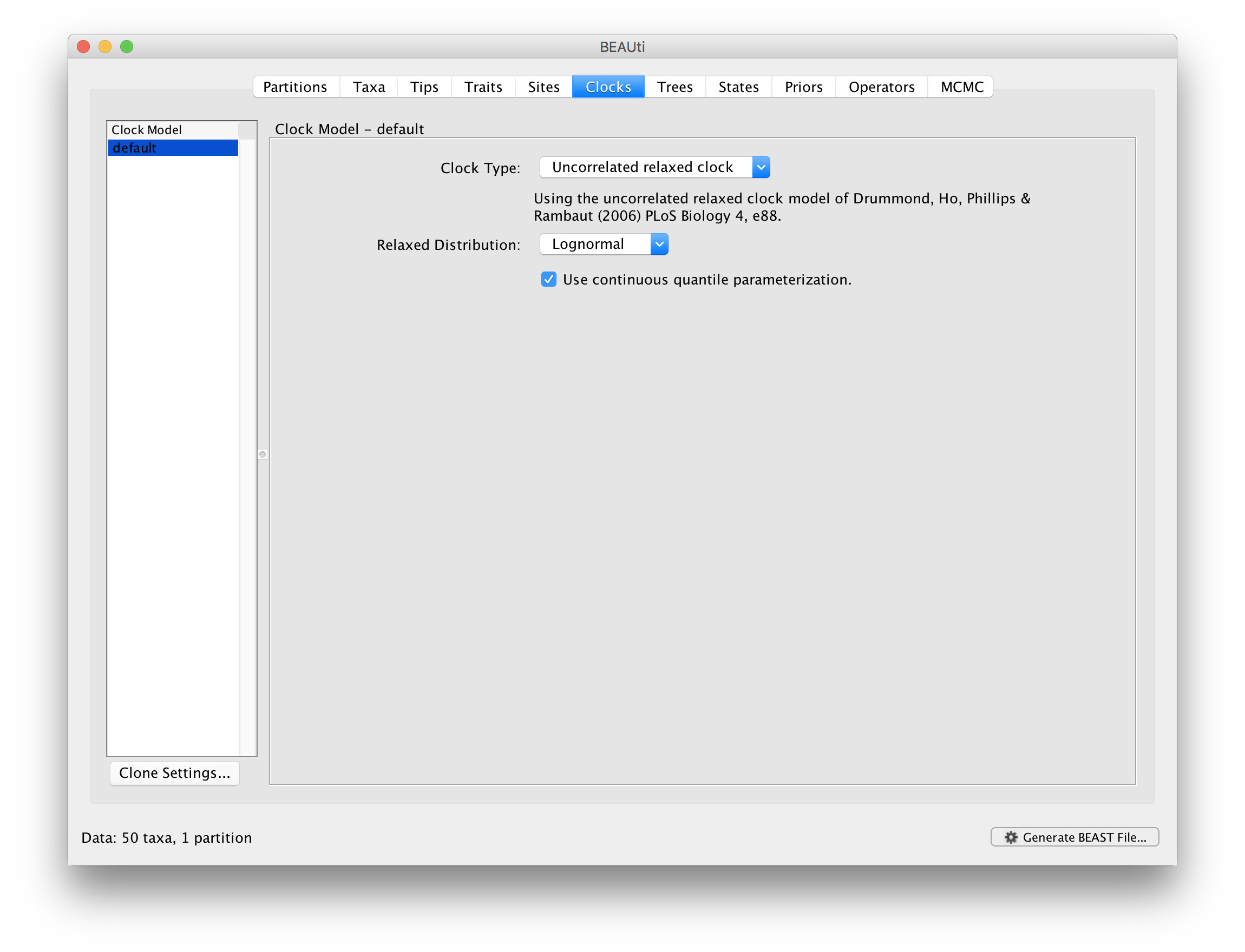
1.6 Set a tree model.

As the phylogenetic tree is built through a coalescent approach, backwards through time based on the genetic diversity at tips/samples, you can will need to set a model for the demographic history of the population that describes the effective population size through time. For example, ‘Constant size’ will state that the effective population size has remained constant through evolutionary time. For the purposes of this exercise, we will choose a constant population size.

In the Trees tab, select ‘Coalescent: Constant Size’ from the ‘Tree Prior’ dropdown box.

Note: You can also input a starting tree on which BEAST will base the topology of the Bayesian tree. This may be a neighbor-joining or parsimony tree and can speed up the analysis by approximating the topology as a prior. We will start with a random tree.

The 'States', 'Priors’ and 'Operators' tabs allow us to specify whether to reconstruct sequences, set specific priors for each parameter, and to specify which operators to include in the output log file. We will leave all these as default values.

1.7 Define the length of the MCMC chain

Finally, the ‘MCMC’ tab is where we will define the steps in the MCMC chain that is used to construct trees. Here we are interested in the length of the chain. This is the number of iterations (number of steps in the random walk) the program will go through to converge on the best tree topology. The higher this number, the more support there will be for the final tree and the more chance of convergence.

Define the length of the chain by typing '10000000' in the 'Length of chain' box.

The name of the output files can be specified here. This will determine the names of the files that will be created after the BEAST run, .log, .trees, and .ops. The output file from BEAUti will be a .xml file for BEAST input. We will call this H1N1.flu.2009, so type this in the ‘File name stem’ box, if it doesn’t already appear there.

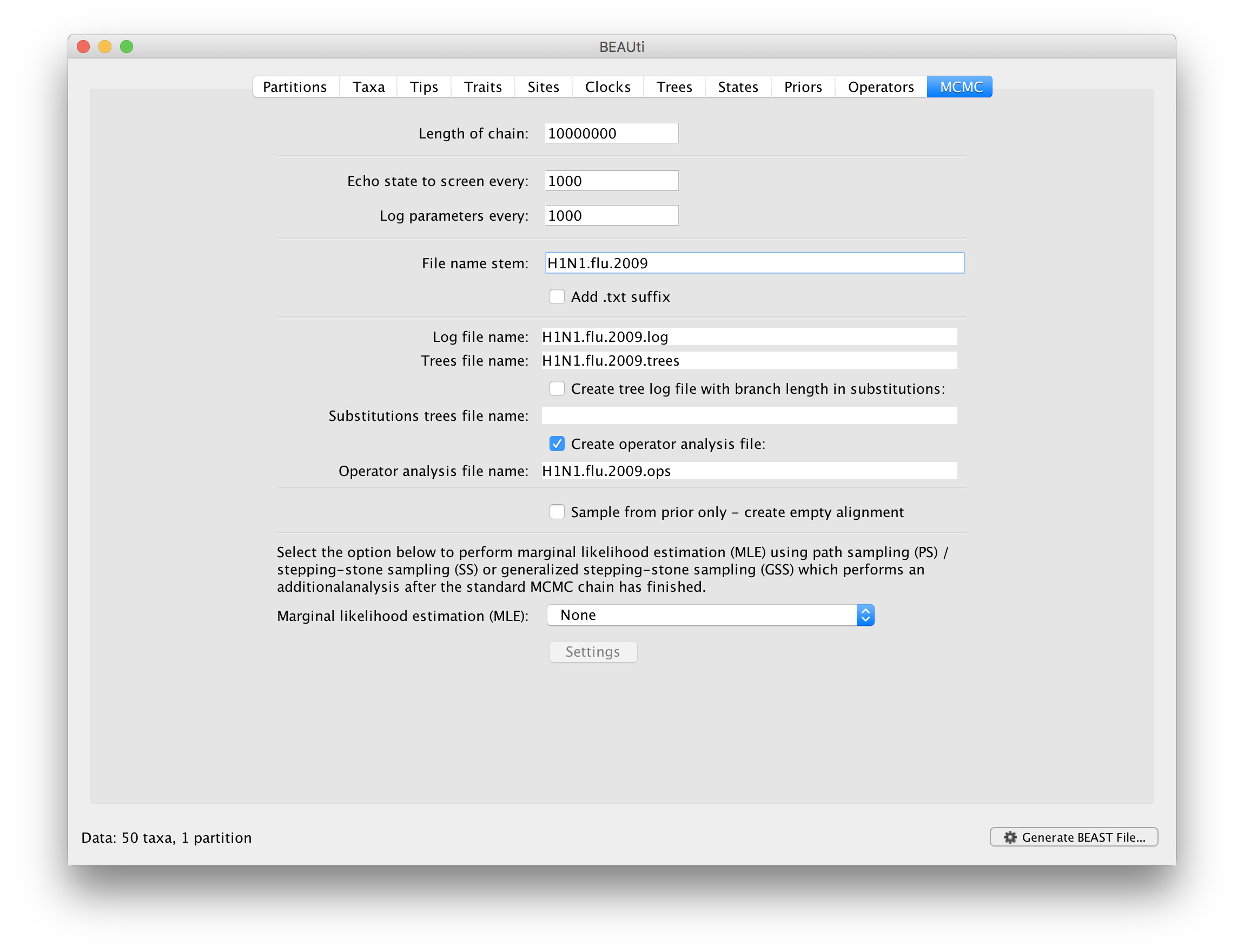
Then click on the Generate BEAST file button at the bottom right of the screen to generate the .xml file that will be used as the input for BEAST.

1. Running the BEAST analysis BEAST can be run on the command line or through the desktop application. We will run BEAST on command line.

To run BEAST, open up a terminal and make sure you are in the folder containing your .xml file from the BEAUti output and type:

beast H1N1.flu.2009.xml

This will create three files; .log, .trees, and .ops, with the “H1N1.flu.2009.” prefix.

1. Evaluating your BEAST run Open the program TRACER by typing tracer. This will allow you to check the output from BEAST and determine how effectively the MCMC has mixed, i.e. how close it is to reaching a steady state (converging). This can be used to manually evaluate the performance of the BEAST run.

Load in the ‘H1N1.flu.2009.log’ file to Tracer to see the output.

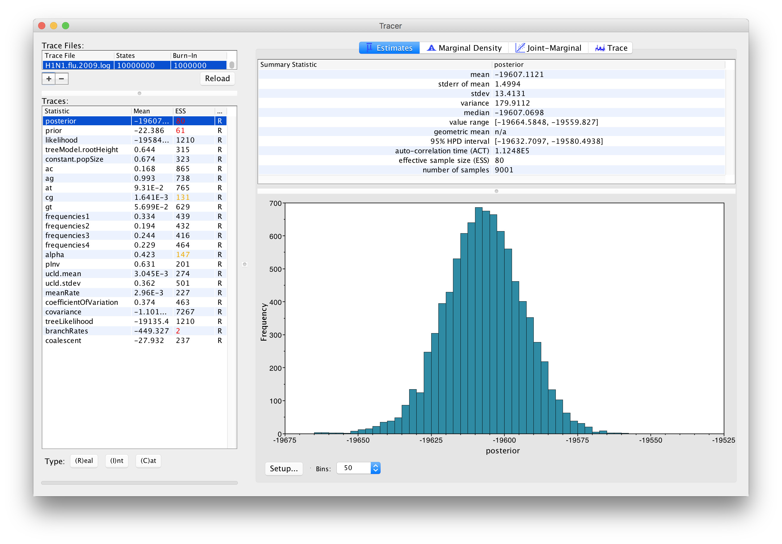
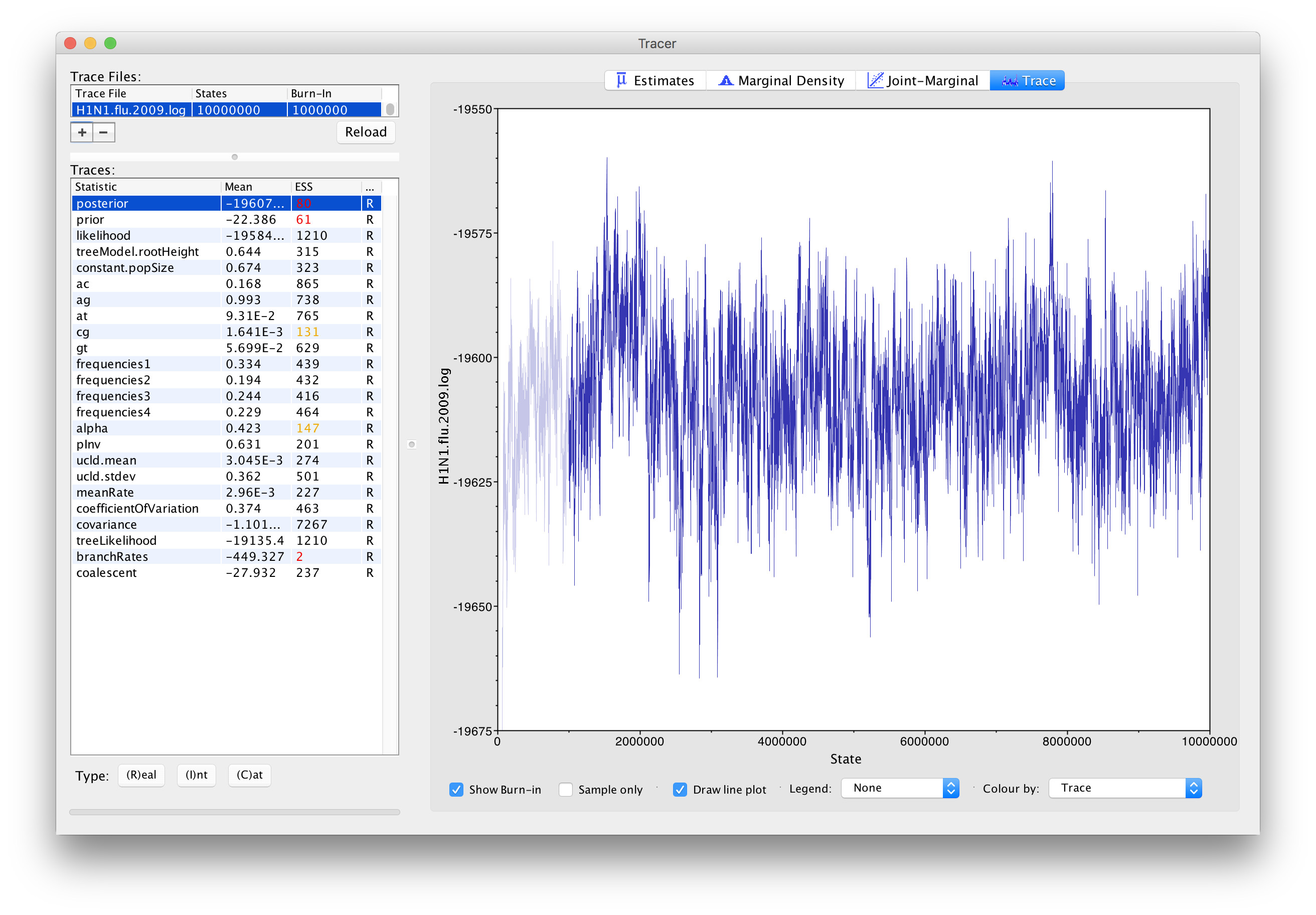
Here we want to look at the ESS score. This is the Effective Sample Size, which is a measure of the number of effectively independent draws from the posterior distribution that the Markov chain is equivalent to. Low scores are highlighted in red, with scores >200 considered sufficient to demonstrate good mixing.

To increase ESS scores, you can run the analysis for longer (more MCMC iterations), or do multiple independent runs that can be combined with the program LogCombiner. Very low scores for many parameters may though suggest that the prior parameters are not a good fit and should be varied.

In our data, we can see that most values are over 200, with only the prior and posterior values highlighted in red. Looking at the “Trace” of the MCMC though, we can see that it remaining reasonably steady around -19600 for the prior parameter, suggesting that this support will increase (ESS will increase) if the MCMC chain was longer.

1. Producing a single phylogenetic tree

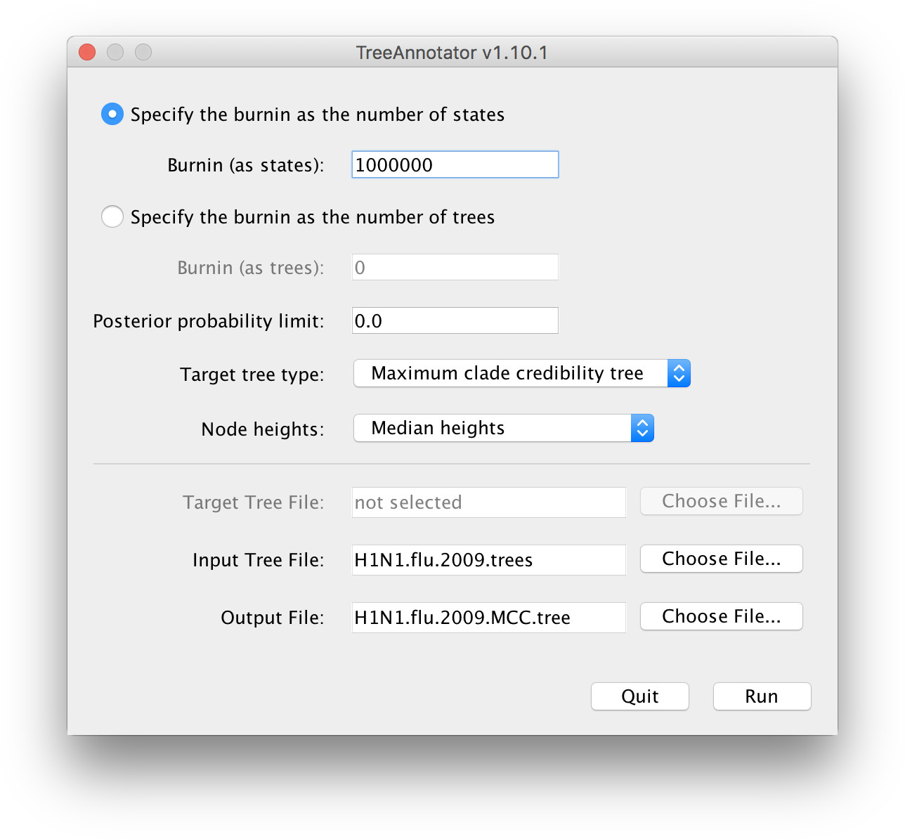
The program TreeAnnotator summarises the sample of trees produced by BEAST (in the .tree file) onto a single maximum clade credibility tree. The posterior probabilities of the nodes in the target tree, the posterior estimates and HPD limits of the node heights and (in the case of a relaxed molecular clock model) the rates, are shown.

Load in the ‘H1N1.flu.2009.trees’ file to TreeAnnotator through Choose File… in Input Tree File. Select what to the call the output file, e.g. H1N1.flu.2009.tre

You can also set the number of burnin states (The number of initial MCMC runs to discard).

Then select Runto produce a single maximum clade credibility tree.

---

Calendar